Neyman–Pearson lemma

In statistics, the Neyman-Pearson lemma, named after Jerzy Neyman and Egon Pearson, states that when performing a hypothesis test between two point hypotheses H₀: θ = θ₀ and H₁: θ = θ₁, then the likelihood-ratio test which rejects H₀ in favour of H₁ when

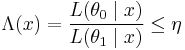
$\Lambda(x)=\frac{ L( \theta _{0} \mid x)}{ L (\theta _{1} \mid x)} \leq \eta$

where

$P(\Lambda(X)\leq \eta|H_0)=\alpha$

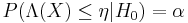
is the most powerful test of size α for a threshold η. If the test is most powerful for all $\theta_1 \in \Theta_1$ , it is said to be uniformly most powerful (UMP) for alternatives in the set $\Theta_1 \,$ .

In practice, the likelihood ratio is often used directly to construct tests — see Likelihood-ratio test. However it can also be used to suggest particular test-statistics that might be of interest or to suggest simplified tests — for this one considers algebraic manipulation of the ratio to see if there are key statistics in it is related to the size of the ratio (i.e. whether a large statistic corresponds to a small ratio or to a large one).

1 Proof
2 Example
3 See also
4 References
5 External links

Proof

Define the rejection region of the null hypothesis for the NP test as

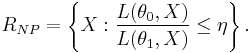
$R_{NP}=\left\{ X: \frac{L(\theta_{0},X)}{L(\theta_{1},X)} \leq \eta\right\} .$

Any other test will have a different rejection region that we define as $R_A$ . Furthermore define the function of region, and parameter

$P(R,\theta)=\int_R L(\theta|x)\, dx,$

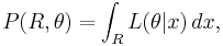
where this is the probability of the data falling in region R, given parameter $\theta$ .

For both tests to have significance level $\alpha$ , it must be true that

$\alpha= P(R_{NP}, \theta_0)=P(R_A, \theta_0) \,.$

However it is useful to break these down into integrals over distinct regions, given by

$P(R_{NP} \cap R_A, \theta) %2B P(R_{NP} \cap R_A^c, \theta) = P(R_{NP},\theta) ,$

and

$P(R_{NP} \cap R_A, \theta) %2B P(R_{NP}^c \cap R_A, \theta) = P(R_A,\theta).$

Setting $\theta=\theta_0$ and equating the above two expression, yields that

$P(R_{NP} \cap R_A^c, \theta_0) = P(R_{NP}^c \cap R_A, \theta_0).$

Comparing the powers of the two tests, which are $P(R_{NP},\theta_1)$ and $P(R_A,\theta_1)$ , one can see that

$P(R_{NP},\theta_1) \geq P(R_A,\theta_1) \text{ if, and only if, } P(R_{NP} \cap R_A^c, \theta_1) \geq P(R_{NP}^c \cap R_A, \theta_1).$

Now by the definition of $R_{NP}$ ,

$P(R_{NP} \cap R_A^c, \theta_1)= \int_{R_{NP}\cap R_A^c} L(\theta_{1}|x)\,dx \geq \frac{1}{\eta} \int_{R_{NP}\cap R_A^c} L(\theta_0|x)\,dx = \frac{1}{\eta}P(R_{NP} \cap R_A^c, \theta_0)$

$= \frac{1}{\eta}P(R_{NP}^c \cap R_A, \theta_0) = \frac{1}{\eta}\int_{R_{NP}^c \cap R_A} L(\theta_{0}|x)\,dx \geq \int_{R_{NP}^c\cap R_A} L(\theta_{1}|x)dx = P(R_{NP}^c \cap R_A, \theta_1).$

Hence the inequality holds.

Example

Let $X_1,\dots,X_n$ be a random sample from the $\mathcal{N}(\mu,\sigma^2)$ distribution where the mean $\mu$ is known, and suppose that we wish to test for 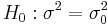$H_0:\sigma^2=\sigma_0^2$ against 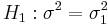$H_1:\sigma^2=\sigma_1^2$ . The likelihood for this set of normally distributed data is

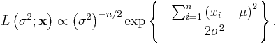
$L\left(\sigma^2;\mathbf{x}\right)\propto \left(\sigma^2\right)^{-n/2} \exp\left\{-\frac{\sum_{i=1}^n \left(x_i-\mu\right)^2}{2\sigma^2}\right\}.$

We can compute the likelihood ratio to find the key statistic in this test and its effect on the test's outcome:

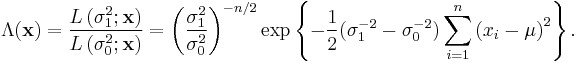
$\Lambda(\mathbf{x}) = \frac{L\left(\sigma_1^2;\mathbf{x}\right)}{L\left(\sigma_0^2;\mathbf{x}\right)} = \left(\frac{\sigma_1^2}{\sigma_0^2}\right)^{-n/2}\exp\left\{-\frac{1}{2}(\sigma_1^{-2}-\sigma_0^{-2})\sum_{i=1}^n \left(x_i-\mu\right)^2\right\}.$

This ratio only depends on the data through $\sum_{i=1}^n \left(x_i-\mu\right)^2$ . Therefore, by the Neyman-Pearson lemma, the most powerful test of this type of hypothesis for this data will depend only on $\sum_{i=1}^n \left(x_i-\mu\right)^2$ . Also, by inspection, we can see that if $\sigma_1^2>\sigma_0^2$ , then $\Lambda(\mathbf{x})$ is an increasing function of $\sum_{i=1}^n \left(x_i-\mu\right)^2$ . So we should reject $H_0$ if $\sum_{i=1}^n \left(x_i-\mu\right)^2$ is sufficiently large. The rejection threshold depends on the size of the test. In this example, the test statistic can be shown to be a scaled Chi-square distributed random variable and an exact critical value can be obtained.

References

Jerzy Neyman, Egon Pearson (1933). "On the Problem of the Most Efficient Tests of Statistical Hypotheses". Philosophical Transactions of the Royal Society of London. Series A, Containing Papers of a Mathematical or Physical Character 231: 289–337. doi:10.1098/rsta.1933.0009. JSTOR 91247.
cnx.org: Neyman-Pearson criterion

External links

Cosma Shalizi, a professor of statistics at Carnegie Mellon University, gives an intuitive derivation of the Neyman-Pearson Lemma using ideas from economics

Neyman–Pearson lemma

Contents

Proof

Example

See also

References

External links